Development Plans

Timeline

Phase 1

2014:

• December: Project start

• Task 3.1.1: Prototyping and Development Planning

2015:

• January

• Task 3.1.1: Prototyping and Development Planning

• February:

• Task 3.1.1: Development Planning Documentation
• Task 3.1.2: Development

• February-August:

• Task 3.1.2: Development
• Task 3.1.3: Documentation

Git Repository

All code and documentation will be maintained in a git repository.

https://bitbucket.org/nathanielroth/uplan

If you would like access to the code or documentation in its rawest form, please contact Nathaniel Roth at neroth@ucdavis.edu for instructions. On completion of this project the repository will be made publicly accessible.

Overview of the UPlan Process

1. Prepare the Base Geometry (parcel layer, grid, or other polygon layer)

1. Topology (no overlaps)
2. (Optional) Pseudoparcels
3. Make centroid dataset
4. Calculate the portion of the polygons already developed
5. (Optional) Specify polygons to be available for redevelopment

2. Calculate the distance from each attractor to the centroid of each polygon
3. For each time step and subarea

1. Available space for each land use in each polygon

1. Union all constraint layers, calculate the area of each primary polygon in each unique combination of constraints
2. Sum the constraint levels for each constraint to get the reduction factor, and multiply times the proportion of the acreage in each constraint type to get a developable space for each land use.
3. GP is also a constraint for each land use

2. Calculate attractions for each polygon for each land use

1. Specify distance and weights, interpolate weights between each point.
2. Select and apply weights for each attractor to each primary polygon for each layer
3. Sum weights
4. Sort by weights for each land use

3. Allocate

1. By land use priority
2. Iterate down list to select highest weighted parcels

1. Redevelopment processing
2. Mixed use

4. Report, Analyze, and Visualize

1. Report on model success and allocation (or under allocation). This would include reporting on UPlan settings.
2. Analyze results

1. Export to TAZ
2. Zonal Summaries

3. Display Maps

Land Use Demand Calculation Options

Method 1

Example Spreadsheet: LUDemandCalc_Method1.xlsx

LU Method 1

(Updated 4/17 to demonstrate subarea functions and some guidance for table construction.)

Is an expansion on the existing method.

1. Population and Employment are divided into subarea by proportion
2. Population is converted into households
3. Households are divided into density types
4. Households by density type are multiplied by acreage to get total acrage of residential type in the subarea
5. Employees are divided by percentage into type
6. Multiplied by SF/Employee
7. Divided by FAR
8. Converted to total area for employment type
9. Expanded Features:

1. Support for vacant residential housing units
2. Support for Other space accounted for within the land use as a % of the area.

Method 2

Example Spreadsheet: LUDemandCalc_Method2.xlsx

LU Method 2

This method expands slightly on method 1 in calculating the households. At its core, this method switches from using population as the primary variable to households. This could also be done as a HU with the addition of a # vacant by HU type. Employment is calculated identically to Method 1.

1. a total proportion of new HU for each subarea is calculated
2. Each HH has a population per HH
3. Each subarea has a proportion of new HU by type
4. Each subarea has a proportion vacant for each HU type
5. A factor is calculated that represents the proportion of the population represented by each of the HU types, and consequently what percentage of the population that represents.
6. This factor is then used to calculate the number of new households and housing units (accounting for HU vacancy) these represent
7. And is multiplied by the acres per HU to get a total number of acres

Method 3

This method is more complex and requires human interaction. However, it allows for mixed use, variable population per household, vacant unit rates, vacant land rates.

Example Spreadsheet: LUDemandCalc_Method3.xlsx

LU Method 3

1. Land use values are established (for each LU type): HU per net acre, PPHH, UnitVacancy rate, % of each employment type, SF/Emp for each emp type, Employment FAR, and % vacant land.
2. From this the building space, ave. SF/emp, Gross Emp/ac, Gross du/ac, Gross occ unit/ac, gross pop/ac, gross emp (by type) per acre are calculated
3. Given targets for population growth and employment growth, a human specifies the ratio of land area across all land uses to achieve the targeted population and employment growth. Note, that there is unlikely to be a single perfect answer to this ratio. These calculations are largely based on accommodating the population and adjusting the land use mixture to match the employment target as closely as possible.

Time Steps:

A UPlan run may be divided into multiple time steps. These will represent specified “break points” between the start date for the UPlan run, and the final end date. For example instead of running UPlan from 2015-2050 in a single step, it could be broken into 2015-2025, 2025-2035, and 2035-2050. Each of these time steps will have potentially independent general plans, constraints, and attracters in addition to the independent demand for each land use. It will be possible to have independent settings for each land use in each time step, though this should be approached with caution.

Subareas:

The use of subareas will allow the application of control totals to subdivide the total growth into geographic areas within the study area boundary. Within each time step a distinct distribution of each land use into each subarea will be specifiable. For example “Subarea 1” could be forced to accommodate 50% of the new residential units, while “Subarea 2” receives 30% and “Subarea 3” gets 20%.

General Plans:

Each time step can have an independent general plan layer.

Constraints:

Each constraint layer (a replacement for the masks used in prior versions of UPlan), will have a % constraint for each land use. The constraints will be unioned and the percent constraint for each land use will be summed for each resulting polygon. These will then be unioned back to the primary layer the amount of space available in each polygon will be recalculated. The developable space will be calculated as (1-%constraint)*acres where the % constraint is the sum of all constraints for that land use in that polygon. A 100% constraint is the equivalent of the current mask.

For example: given a 1 acre parcel, with two constraint (one with at 50% constraint, and the other with 25%) layers that over lap it so that 25% of the original polygon has both constraints overlapping it, 25% has only the 50% constraint, 25% of it has only the 25% constraint, and 25% has no constraint.

There will then be a quarter acre with no constraint, quarter acre with a 25% constraint(0.1875 Developable Acres (dac)), a quarter acre with 50% constraint( 0.125 dac), and a quarter acre with a 75% constraint (0.0625 dac) meaning that the original polygon has 0.625 developable acres.

Attracters:

Attraction layers can be specified for each land use in each time step. For each attracter a series of distances and weights (called weight points for simplicity) are specified. For example, at a distance of 0 miles from the attracter (hypothetically a city limit) the weight may be 20, at a distance of 1 miles the weight might be 10, and at a distance of 5 miles the weight would be 0. These weight points create a series of distance ranges and allow for the interpolation of weights between each pair of sequential points.

Attracter weights can be negative values replicating the function of discouragers without needing to duplicate code or input effort.

The process of calculating a net attraction of a polygon for a land use (in a time step) is as follows:

1. Calculate the distance from the centroid of the polygon (BaseGeom_cent) to the nearest feature in each attracting layer. These results are assembled into a table containing one row for each polygon, and columns/fields that identify the polygon, and the shortest distance to each attraction layer.
2. Each sequential set of weight points are reformulated to create a linear function of the weight with respect to the distance. i.e. for all polygons between 0 and 1 mile from the city limit the weight would be: weight = -10*(distance) + 20
3. These functions are applied to the distances to generate a weight provided by each attracter for each land use to each polygon.
4. The attracters are summed for each land use to create a net attraction.

Allocation Process:

The following will occur simultaneously for each land use:

Allocation: 1. Calculate the attraction weight for each polygon with developable space. 2. Sort in descending order. 3. Loop through the polygons adding up the available space until the next polygon goes over the needed space. 4. Then update all of the earlier polygons to show 100% development and apply the needed percentage to the polygon that makes up the last to achieve the correct acreage. 5. If all available space is exhausted, mark all available polygons as 100% developed and report the unallocatable space.

Evaluation: Following the allocation of each land use, all of the results are collected, then on a polygon by polygon basis the land uses allocated to it are evaluated for conflicts accounting for allowed mixed uses. Any conflicts are resolved by removing the lowest priority land uses until a permitted combination is allowed. The acres that are removed from each land use are added to a list of land use demand that requires reallocation and following the evaluation of all polygons, another iteration of the allocation is run using an updated list of available space for each polygon.

The Allocate-Evaluate loop continues until either all land use demand has been allocated, or all available space for each land use has been consumed.

Random Allocation:

Random allocation will be similar to the existing UPlan where the development will be limited by contstraints and general plan, but attractions will be ignored infavor of a random allocation mechanism.

Weighted Random Allocation:

Convert the weights to a -10 to 10 scale (which we’ll use informally as its Utility) with configurable mean and standard deviation, then apply a binomial logit function to each polygon’s Utility. This is an application of the logistic function (http://en.wikipedia.org/wiki/Logistic_regression) in which the probability of an event occurring can be related a function that determines its Utility. In this case, the “event” will be that polygon getting developed by the land use.

See the table below for the probabilities associated with each level of utility.

Logit Probabilities

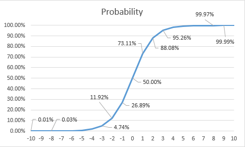
Utility	Probability
-10	0.005%
-9	0.012%
-8	0.034%
-7	0.091%
-6	0.247%
-5	0.669%
-4	1.799%
-3	4.743%
-2	11.920%
-1	26.894%
0	50.000%
1	73.106%
2	88.080%
3	95.257%
4	98.201%
5	99.331%
6	99.753%
7	99.909%
8	99.966%
9	99.988%
10	99.995%

Based on these probabilities for each polygon, a random number generator can be used as part of a Monte Carlo simulation to select polygons to be developed in a weighted random operation.

Mixed Use:

For each general plan class, sets of land uses can be defined that may be allocated on top of each other. These land uses will not block each other. The final land use for that polygon will be the sum of the contributions from each land use that is permitted into that location.

Redevelopment:

Each polygon may be given an “existing” population and employment totals. If a polygon with a non-0 total is allocated with a new land use, that total displacement is totalled up, and at the end of the allocation, a new land use total for each is created through applying the demographic settings for that time step and zone and another loop of allocation is conducted (and likely iterated until all growth is allocated). The space needed to accommodate population or employment displaced by redevelopment may be inserted with the mixed use or land use conflict land for subsequent allocations.

Database Structure:

Each File Geodatabase used for a UPlan run will be fully self contained. It will have all settings and data needed to run UPlan including the boundary layers, BaseGeometry layers, attracters, constraints, and general plans.

Key Values: Individual configuration settings. Most of these are primary configurations that stand alone.

• BaseGeom_bnd: name of the base geometry boundary feature class
• BaseGeom_cent: name of the base geometry centroid feature class
• BaseGeom_id: name of the id field to be used in both the BaseGeom_bnd and BaseGeom_cent feature classes.
• BaseGeom_linearunit: the linear unit used in the projection for the BaseGeom_bnd feature class.
• baseGeom_areaunit: the area unit to be used (defaulting to acres)
• SubArea: the name of the feature class defining the subarea. If Null then the entire BaseGeom_bnd will be treated as a single subarea.
• Scenario_name: a name for the scenario
• Scenario_rundate: the date the scenario was last run
• Scenario_user: name of the person conducting the run
• Scenario_notes: notes for the scenario?
• Scenario_fullrun: True/False was the run successful?
• Scenario_fullallocation: True/False was full allocation achieved?
• DistMode: The mode to be used for calculating the distances between attractors and base geometry centroids. This could be either ‘GenerateNear’ or ‘RasterEuc’ If ‘GenerateNear’ is selected, then the user will have to have an ArcGIS Advanced license. If ‘RasterEuc’ is selected then the user will need a Spatial Analyst extension license. Note: I’ve just come across a possible way to avoid the licensing needs, but it probably won’t be as fast as either of these two, so it might create a third option
• Redev: True/False Perform redevelopment operation.
• Redev_sa_mode: Define how redevelopment behaves with respect to subareas. Are population and employment replaced into the same subarea, or do they follow the primary population method which might distribute them to other subareas.

Time Steps:

• TS_order: The order of the time step to be executed
• TS_short: short name for the time step to be used within table and field names. This will be used as a value for look up tables or other actions within UPlan. Ideally it will be <4 characters with no spaces or special characters.
• TS_long: Long name for the time step to be used for human consumption. This can have spaces or special characters.

SubAreas:

• SA_short: short name for the subarea. This will be used as a value for look up tables or other actions within UPlan. Ideally it will be <4 characters with no spaces or special characters.
• SA_long: long name for the subarea. This can have spaces or special characters.

Redevelopment: This optional inclusion requires that a table with the same BaseGeom_id exist, and that it have a numeric field with for existing population and existing employment. * rd: the name of the feature class or table providing population and employment totals * rd_pop: the name of the field providing a population total for that BaseGeom_id * rd_emp: the name of the field providing a employment total for that BaseGeom_id

Land Uses:

• LU_priority: The order in which land uses will be given access to land.
• LU_short: short name for the land use. This will be used as a value for look up table or other actions within UPlan. Ideally it will be <4 characters with no spaces or special characters.
• LU_long: long name for the land use. This can have spaces or special characters.
• LU_allocmethod: Specifies how the land use will be allocated. The options being considered are normal (using deterministic weights), random (fully random), weighted random (binomial logit formulation).
• LU_color: a color for displaying the land use

Land Use Properties: (for output calculations)

• LU_short: Key linking back to the land uses list.
• gross_du_density: the gross density of dwelling units (occupied and unoccupied housing units)
• gross_hh_density: the gross density of households (occupied housing units)
• gross_emp_density: the gross employment density (possible extra types by type of employment through a linked table)
• gross_emp_sf_density: the density of employment square footage (possible extra types by type of employment through a linked table)

Land Use Demand Properties: still in progress, and potentially very flexible. These will be the inputs used to generate the Land Use Properties (above). See the discussion about land use demand methods below. These values will not be used directly by UPlan.

Land Use Demand: The demand for land use will be measured in acres.

• ts: TimeStep, linked to TS_short
• sa: Subarea, linked to SA_short
• lu: The land use, linked to LU_short
• demand: acres of the land use demanded.

General Plans:

• ts: TimeStep, linked to TS_short
• gp: feature class name for the general plan
• gp_field: the field name providing the general plan class

General Plans-Land Use:

• ts: TimeStep, linked to TS_short
• gp_class: the gp class contained within the gp_field(above)
• lu: the LU_Short for the permitted land use

Mixed Use: still under development and may change

• ts: TimeStep, linked to TS_short
• gp_class: the gp class contained within the gp_field(above)
• mu_group: This will need to be constructed to hold groupings of land uses that are permitted to occur together in this general plan class. This may be needed to handle the one to many relationship between gp_class and permitted land uses.
• lu: the LU_Short for the permitted land use.

Constraints: feature classes to be used as constraints

• ts: TimeStep, linked to TS_short
• const_short: feature class name to be used as a constraint

Constraint Levels: the level of constraint to be applied to each land use

• ts: TimeStep, linked to TS_short
• const_short: the constraint feature class name
• lu: The land use, linked to LU_short
• const_weight: the weight 0.0 to 1.0 that will reduce the availability of impacted area to the specified land use.

Attracter: feature classes to be used as attracter

• ts: TimeStep, linked to TS_short
• att_short: feature class name to be used as an attracter.

Attraction Weights: the level of attraction to be applied to each land use

• ts: TimeStep, linked to TS_short
• att_short: the attraction feature class name
• lu: The land use, linked to LU_short
• att_dist: the distance from the attracter at which the weight will be applied
• att_weight: the weight that will be applied for attraction purpose at the distance specified in att_dist. The weight can be either positive or negative (allowing for discouragement based on distance).

Logit Parameters: Still in development. Parameters that are needed to handle random weighted allocation. These will be used to convert weights into utils for the random weighted allocation.

• ts: TimeStep, linked to TS_short
• lu: The land use, linked to LU_short
• Util_mean: the mean utility
• Util_sd: desired standard deviation of the utilities

Technologies

Development Platform Alternatives

Esri

(Selected Option)

Type: ArcGIS Extension

Model Code: python 2.7

GUI: C# With significant portions in a Python Toolbox

Data Storage: File Geodatabase

Django

Type: Web App

Model Code: Python 2.7 or 3.4

GUI: Django

Data Storage: PostGIS

QGIS Plug-in

Type: Plug-in

Model Code: Python 2.7 or 3.4

GUI: QT

Data Storage: PostGIS

Discussion of Development Options

ESRI ESRI is far more familiar and comfortable to most of our potential user base. However, some of the components we would want to use require licensing beyond basic ArcGIS desktop. For example: Calculating distances from parcels to the nearest road requires the Near, or Near Table tools which both require the Advanced licensing level. An alternate method using the raster euclidean distance functions will require the spatial analyst extension. Note: I’ve just come across a possible way to avoid the licensing needs, but it probably won’t be as fast as either of these two, so it might create a third option that doesn’t have additional licensing requirements

Django Is basically a web application, and it could be fairly easily configured to operate on a server as an externally accessible site with permissions. PostGIS has substantial spatial analysis and indexing capabilities that allow for the rapid calculation of distances between large numbers of features

It could also have other interfaces built ontop of it or plug-ins to other applications such as QGIS or ArcGIS

QGIS This would work much like the Esri extension but with QGIS as the primary platform and PostGIS as the back end.

Survey Response

In late February, a short survey looking for feedback on several key design choices for UPlan was sent to a list of about 15 past and present users. As of Feb. 26, there were 11 responses.

Question 1. Which best describes your past UPlan use?

• Extensive experience (used on multiple projects with minimal outside help): 5 or 45.45%
• Substantial experience (used in the past with moderate outside help):4 or 36.36%
• Basic experience (have used, but with a lot of help): 2 or 18.18%

Question 2. When using UPlan would you rather...

• Have UPlan in the Esri GIS environment (and have to maintain either a ArcGIS Advanced license or a Spatial Analyst Extension): 9 or 90%
• Use UPlan as a plug-in to QGIS (and have to learn QGIS and some PostGIS): 0
• Use UPlan as a web application (and have to learn PostGIS, and some Django web and server administration): 1 or 10%

Question 3. Which current features are/were most important to you?

• Simple demographics: 3.82
• Requires only basic GIS data: 3.36
• Deterministic Allocation: 3.64
• Default TAZ Export: 2.0
• Custom TAZ Export: 2.18

Question 4. Which features would you most like to see added?

• Vertical Mixed Use: 5.0
• Improved Redevelopment: 3.64
• Weighted Random Allocation: 3.0
• Time Steps: 4.18
• Statistical Calibration of Weights: 3.18
• Model Validation: 2.0

Question 5. Any other suggestions you have for improving UPlan.

• The buttons in Questions 3&4 don’t seem to be working; they just default to numerical order. In general I’d love to see UPlan remain as user-friendly and flexible as possible. Requiring users to know programming doesn’t seem like a good idea. Vertical mixed use and time steps both seem like good ideas.
• My ranking in questions 3 and 4 are only really valid for the top rankings. Otherwise I am indifferent. Also, I did not answer question 2 because my answer would be ‘most cost effective option.’ If QGIS is easy enough to learn and will cost less than maintaining an advanced license, then that would be my choice. Although I imagine that UPlan will maintain its largest user base if it is in the Esri environment.
• A more straight-forward way to accommodate “over-building” of residences due to intentionally unoccupied dwelling units (vacation homes, etc), particularly as the percentage of those homes can be statistically derived for distinct geographic sub-areas.
• Optional input mechanisms for assessor land and improvement values ratios for parcels and/or land price contours that can automate attractiveness for specific use intensities.
• better linking of UPLAN land use categories to traffic model variables AND census stats AND labor market data ...
• I would, of course, like to see all of these!

Development

As of the middle of February, the sentiment that has been voiced has been in favor of developing UPlan within the Esri environment.

The current versions of UPlan already require that the user have a license for Spatial Analyst. Under small government licensing, the cost of maintaining the spatial analyst license, or maintaining a single seat of ArcGIS Advanced are effectively equivalent.

Initial prototype development has also gone very smoothly within the Esri environment. Based on this, we will be proceeding with development in the Esri programming environment.

The code will be divided into two primary components: the User Interface (UI), and the operational code (arcpy).

User Interface

The user interface will be written in C# as an ArcGIS Desktop Add-in. At a minimum it will include a custom toolbar providing access to the various UPlan tools. These tools will include functionality to prepare the “base geometry” layers, set up a geodatabase to contain a run, import layers into that geodatabase, configure the model inputs, initiate the run, and report on and analyze the outputs.

Portions of the supporting code will be simplified to work as tools within a Python Toolbox (http://resources.arcgis.com/en/help/main/10.2/index.html#//001500000022000000 ) for ease of access and to make their maintanance as simple as possible.

Operational Code

The operational code will be written in Python making use of Esri’s arcpy libraries to perform geoprocessing operations. This code will be subdivided into functional areas each of which will have its own Python module (a .py file containing code).

Independent modules have been created to manage processes that control the configuration settings for UPlan, data preparation, utility functions, prepare general plan data, calculate the effects of constraint layers, calculate attraction weights, and control allocation of new land use. Additional modules will be created to handle the calculation of demand for each land use, report generation, results analysis, and visualization. Each module will have one, or possibly a few primary functions that are called in order to run UPlan.

As presently written the general plan, constraints, and attraction modules primary purpose can be executed in any order (or possibly simultaneously), because they are not dependent on each other. In general the work flow will follow the following pattern: Data preparation, run configuration, (general plan, constraints, attractions), allocation, (visualization, analysis, reports). The modules grouped in () could be run in any order as long as the prior sections have been completed.

Supporting Utilities

The tools needed to run UPlan will need several utilities to support their use, these will include tools for preparing data sets and analyzing results.

Base Geometry Preparation

The Base Geometries for UPlan will need to be prepared ahead of any new model run. These base geometries will serve as the spatial units that growth will be allocated to. In many ways they can be thought of as parcels, though as will be discussed a true parcel layer will probably have some disadvantages compared to a layer that has been processed in several ways.

• First, the base geometry layer will need to exist in two forms, the primary and more important is as polygon boundaries. This will be referred to in the code as BaseGeom_bnd.
• The base geometry boundary layer must be in a correctly projected spatial reference. i.e. State Plane, California Albers, UTM, Web Mercator. This will allow the easy calculation of areas and distances.
• Each base geometry must have a unique id (BaseGeom_id) that can be used by UPlan. For efficiency this should be a long integer.
• Each base geometry will have a calculated acreage.
• Also for efficiency, the base geometry should have minimal additional attributes. All other data general plans, existing land use, attracters, and constraints will have their relationships to the base geometry tracked based on their overlap with the boundaries (or the polygon’s centroid) and recorded based on the polygon id.
• These polygon boundaries must not overlap or that overlapping space will potentially be developable within both polygons. i.e. it could be double counted on allocation.
• Gaps between polygons may not be a critical issue, but should be considered carefully as the space covered by those gaps will be not be considered by UPlan. Some examples of potential gaps would be road rights of way, water bodies, or other completely undevelopable lands. One advantage is that the areas omitted will not be processed by UPlan, possibly increasing run times, though this is likely to be only a very minor benefit unless there are large numbers of polygons.
• The base geometry will be the minimum unit that can be allocated. As a result, large polygons in areas likely to experience development should be subdivided into “pseudo-parcels” that more closely represent the land blocks likely to occur during development. For example, an area that is likely to develop into housing units should be subdivided into polygons that represent only a few housing units.
• An alternate way of constructing base geometries is through the construction of a base geometry that is not based directly on parcels. There are many way that this could happen, but some examples are:

• Building Thiessen or Vornoi polygons (two commonly used names for the same process) from parcel or pseudo-parcel centroids. This would allow for a replication of current parcel locations and sizes without exactly replicating the parcels.
• Constructing a fishnet (see the Create Fishnet tool in ArcGIS). This supports the construction of a grid of equally sized and shaped polygons across the area of analysis and will allow UPlan to closely replicate the behavior of the prior raster based versions of UPlan.
• Hybrid. The use can build their base geometry set through merging other data set, for example, a fishnet could be used to cover rural portions of the county while a parcel data set is used in and around cities or towns.

• A second base geometry data set will be needed that is the conversion of the base geometry boundary layer into centroids. This layer will be used for calculating distances to and from the polygon. It need have only the point (shape field), and the BaseGeom_id. The layer will be referred to in code as BaseGeom_cent.

Tools to be be built for base geometry preparation:

• BaseGeom importer: Import BaseGeom_bnd, check the projection, calculate acreage, create a BaseGeom_id field if one is not already created, and create BaseGeom_cent.
• Thiessen Polygon BaseGeom Tool: Create BaseGeom_bnd from a set of points (which become BaseGeom_cent). Calculate the acreage and ensure consistency in BaseGeom_id. Note, this will require the “Advanced” level licensing for ArcGIS.
• Fishnet BaseGeom Tool: Create BaseGeom_bnd, and BaseGeom_cent based on the Fishnet tool in ArcGIS. Unless feedback suggests an better alternative, the inputs will be a study area boundary data set and a user specified acreage for the polygons in the fishnet.
• Pseudoparcelling Tool: Easily create a possible BaseGeom_bnd from parcel (or other polygon) data by taking a polygon layer where each polygon has a maximum polygon size (acres) and automatically subdivide those polygons until all polygons are below the specified size.

Other Layers

Other layers will require less preparation. They will need to be , checked to make sure that they are in the same projection as the BaseGeom layers, imported to the geodatabase, and will be registered so that the user interface will recognize them and their purpose.

Layer Types:

• General Plan: A general plan layer will need to be registered with the name of field (or fields) containing general plan classes
• Attracter: An attracter will need no additional information for registration. (possible addition: one or more queries allowing for a subset of the data to be used as an attracter). For example you upload one road layer, and use queries to define road classes for separate attraction levels)
• Constraint: A constraint will need no additional information for registration, though it must be a polygon layer. (possible addition: one or more queries allowing for a subset of the data to be used as a constraint). For example you upload one environmental layer, and use queries to define classes for separate constraint levels)
• Subarea: A field to be used to identify subareas must be specified.
• Redevelopment: a layer/table that has the existing population and employment totals for each BaseGeom. This is used as part of the redevelopment function.

Tool to be built for layer import:

• Layer Import: Check projection on the layer, import to geodatabase, and register the layer with UPlan. Inputs will be the layer, the role(s) the layer will be available for, and a limited set of parameters needed for UPlan to use the layer.

Zonal Export (TAZ Export)

Following a model run, the user will be able to specify a new layer (and one or maybe more fields within it) to use to summarize the new growth (acres, persons, housing units (by type), employment space, employees (by type)) for each value in the field. This would be a precursor to the custom TAZ export, and provides all of the functionality in the existing default TAZ export.

Tool to be built for zonal or TAZ summaries

• Zonal Summary: Takes a new layer, and one or more fields. The base geometries with their growth increment (and displaced redevelopment if used) will be summarized by the intersection with the zone layer and then aggregated based on the fields provided as the input.

Custom TAZ Export

This is a replication, though hopefully also a simplification, of the custom TAZ export tool that allows the remapping and addition of UPlan results to an existing base year TAZ dataset. It will have functionality to save the configurations for reuse and will include both the creation of default exports which will apply to all TAZs, and exceptions which allow overriding the settings for individual TAZs.

Custom TAZ export tool

• Custom TAZ Export: Support for remapping the output from the Custom TAZ Export onto an existing TAZ table. This will allow the recombination of residential and employment types into the TAZ table. There will be a default export pattern that will be applied to all TAZs that do not have an exception. Exceptions will allow for targeted re-remapping of the output for individual TAZs. These configurations can be saved for reuse.